The PID controller algorithm involves three separate constant parameters, and is accordingly sometimes called three-term control: the proportional, the integral and derivative values, denoted P, I, and D. Simply put, these values can be interpreted in terms of time: P depends on the present error, I on the accumulation of past errors, and D is a prediction of future errors, based on current rate of change. The weighted sum of these three actions is used to adjust the process via a control element such as the position of a control valve, a damper, or the power supplied to a heating element.
In the absence of knowledge of the underlying process, a PID controller has historically been considered to be the most useful controller.[2] By tuning the three parameters in the PID controller algorithm, the controller can provide control action designed for specific process requirements.
Lets spend few minutes with this very good video:
The Theory:Anatomy Of A Feedback Control System
Here is the classic block diagram of a process under PID Control.
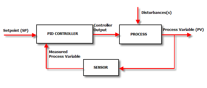
The Setpoint (SP) is the value that we want the process to be.
For example, the temperature control system in our house may have a SP of 22°C. This means that
“we want the heating and cooling process in our house to achieve a steady temperature of as close to 22°C as possible”
The PID controller looks at the setpoint and compares it with the actual value of the Process Variable (PV). Back in our house, the box of electronics that is the PID controller in our Heating and Cooling system looks at the value of the temperature sensor in the room and sees how close it is to 22°C.
If the SP and the PV are the same – then the controller is a very happy little box . It doesn’t have to do anything, it will set its output to zero.
However, if there is a disparity between the SP and the PV we have an error and corrective action is needed. In our house this will either be cooling or heating depending on whether the PV is higher or lower than the SP respectively.
Example:
Let’s imagine the temperature PV in our house is higher than the SP. It is too hot. The air-con is switched on and the temperature drops.
The sensor picks up the lower temperature, feeds that back to the controller, the controller sees that the “temperature error” is not as great because the PV (temperature) has dropped and the air con is turned down a little.
This process is repeated until the house has cooled down to 22°C and there is no error.
Then a disturbance hits the system and the controller has to kick in again.
In our house the disturbance may be the sun beating down on the roof, raising the temperature of the air inside.
So that’s a really, really basic overview of a simple feedback control system. Sounds dead simple eh?
Understanding the controller
Unfortunately, in the real world we need a controller that is a bit more complicated than the one described above, if we want top performance form our loops.
To understand why, we will be doing some “thought experiments” where we are the controller. When we have gone through these thought experiments we will appreciate why a PID algorithm is needed and why/how it works to control the process.We will be using the analogy of changing lanes on a freeway on a windy day. We are the driver, and therefore the controller of the process of changing the car’s position.Here’s the Block Diagram we used before, with the labels changed to represent the car-on-windy-freeway control loop.
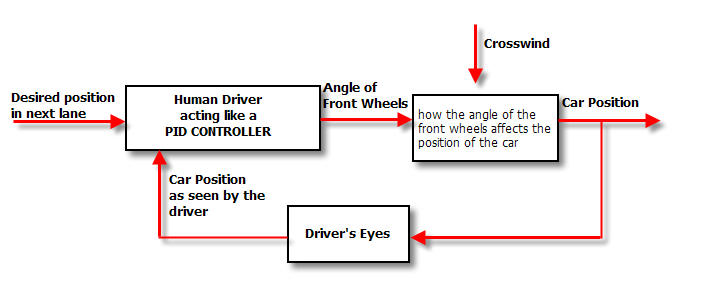
Notice how important closing the feedback loop is. If we removed the feedback loop we would be in “open loop control”, and would have to control the car’s position with our eyes closed!
Thankfully we are under “Closed loop control” -using our eyes for position feedback.
As we saw in the house-temperature example the controller takes the both the PV and SP signals, which it then puts through a black box to calculate a controller output. That controller output is sent to an actuator which moves to actually control the process.
We are interested here in what the black box actually does, which is that it applies 1, 2 or 3 calculations to the SP and Measured PV signals. These calculations, called the “Modes of Control” include:
- Proportional (P)
- Integral (I)
- Derivative (D)
The World Famouse PID Controller
Here’s a simplified block diagram of what the PID controller does:
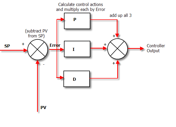
It is really very simple in operation. The PV is subtracted from the SP to create the Error. The error is simply multiplied by one, two or all of the calculated P, I and D actions (depending which ones are turned on). Then the resulting “error x control actions” are added together and sent to the controller output.
These 3 modes are used in different combinations:
- P – Sometimes used
- PI – Most often used
- PID – Used
- PD – rare as hen’s teeth but can be useful for controlling servomotors.
Derivatives
Go into the control room of a process plant and ask the operator:
“What’s the derivative of reactor 4’s pressure?”
And the response will typically be:
“Bugger off smart arse!”
However go in and ask:
“What’s the rate of change of reactor 4’s pressure?”
And the operator will examine the pressure trend and say something like:
“About 5 PSI every 10 minutes”
He’s just performed calculus on the pressure trend! (don’t tell him though or he’ll want a pay raise)
So derivative is just a mathematical term meaning rate-of-change. That’s all there is to it.
Integrals without the Math
Is it any wonder that so many people run scared from the concept of integrals and integration, when this is a typical definition?
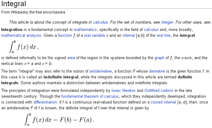
hmmmm…what??
Here’s a plain English definition:
The integral of a signal is the sum of all the instantaneous values that the signal has been, from whenever you started counting until you stop counting.
So if you are to plot your signal on a trend and your signal is sampled every second, and let’s say you are measuring temperature. If you were to superimpose the integral of the signal over the first 5 seconds – it would look like this:
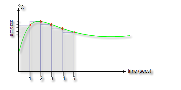
The green line is your temperature, the red circles are where your control system has sampled the temperature and the blue area is the integral of the temperature signal. It is the sum of the 5 temperature values over the time period that you are interested in. In numerical terms it is the sum of the areas of each of the blue rectangles:
(13 x 1)+(14×1)+(13×1)+(12×1)+(11×1) = 63 °C s
The curious units (degrees Celsius x seconds) are because we have to multiply a temperature by a time – but the units aren’t important.
As you can probably remember from school –the integral turns out to be the area under the curve. When we have real world systems, we actually get an approximation to the area under the curve, which as you can see from the diagram gets better, the faster we sample.
Proportional Control
Here’s a diagram of the controller when we have enabled only P control:
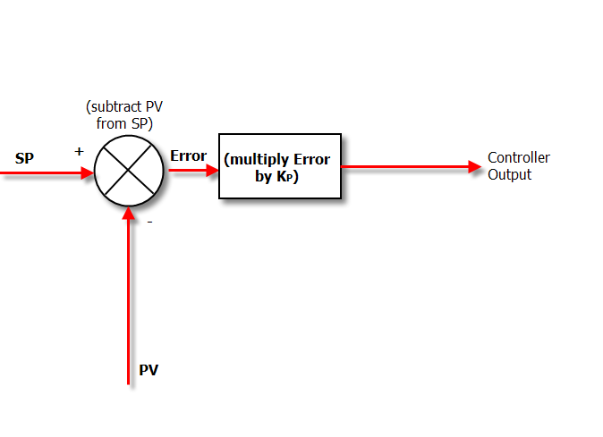
In Proportional Only mode, the controller simply multiplies the Error by the Proportional Gain (Kp) to get the controller output.
The Proportional Gain is the setting that we tune to get our desired performance from a “P only” controller.
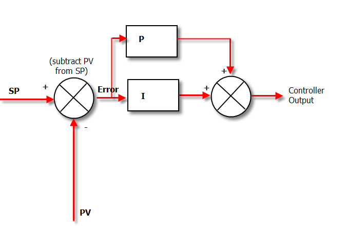
The P+I Controller
If we put Proportional and Integral Action together, we get the humble PI controller. The Diagram below shows how the algorithm in a PI controller is calculated.
The tricky thing about Integral Action is that it will really screw up your process unless you know exactly how much Integral action to apply.
A good PID Tuning technique will calculate exactly how much Integral to apply for your specific process – but how is the Integral Action adjusted in the first place?
Adjusting the Integral Action
The way to adjust how much Integral Action you have is by adjusting a term called “minutes per repeat”. Not a very intuitive name is it?
So where does this strange name come from? It is a measure of how long it will take for the Integral Action to match the Proportional Action.
In other words, if the output of the proportional box on the diagram above is 20%, the repeat time is the time it will take for the output of the Integral box to get to 20% too.
And the important point to note is that the “bigger” integral action, the quicker it will get this 20% value. That is, it will take fewer minutes to get there, so the “minutes per repeat” value will be smaller.
In other words the smaller the “minutes per repeat” is the bigger the integral action.
To make things a bit more intuitive, a lot of controllers use an alternative unit of “repeats per minute” which is obviously the inverse of “minutes per repeat”.
The nice thing about “repeats per minute” is that the bigger it is – the bigger the resulting Integral action is.
Derivative Action- Predicting the future!
OK, so the combination of P and I action seems to cover all the bases and do a pretty good job of controlling our system. That is the reason that PI controllers are the most prevalent. They do the job well enough and keep things simple. Great.
But engineers being engineers are always looking to tweak performance.They do this in a PID loop by adding the final ingredient: Derivative Action.So adding derivative action can allow you to have bigger P and I gains and still keep the loop stable, giving you a faster response and better loop performance.
If you think about it, Derivative action improves the controller action because it predicts what is yet to happen by projecting the current rate of change into the future. This means that it is not using the current measured value, but a future measured value.The units used for derivative action describe how far into the future you want to look. i.e. If derivative action is 20 seconds, the derivative term will project the current rate of change 20 seconds into the future.The big problem with D control is that if you have noise on your signal (which looks like a bunch of spikes with steep sides) this confuses the hell out of the algorithm. It looks at the slope of the noise-spike and thinks:“Holy crap! This process is changing quickly, lets pile on the D Action!!!”And your control output jumps all over the place, messing up your control.
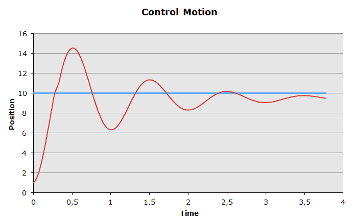
Now, test yourself!:
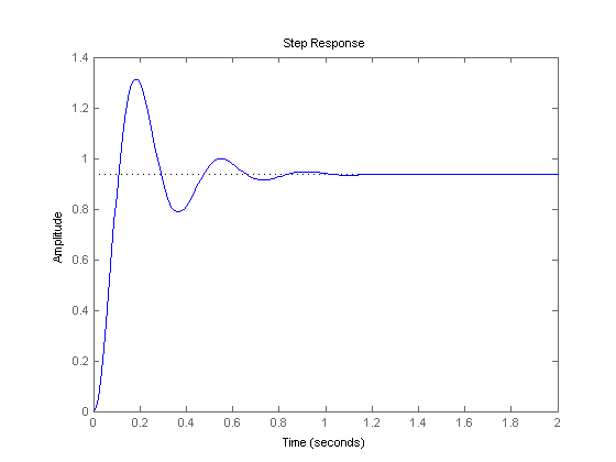
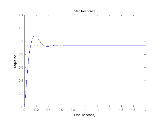
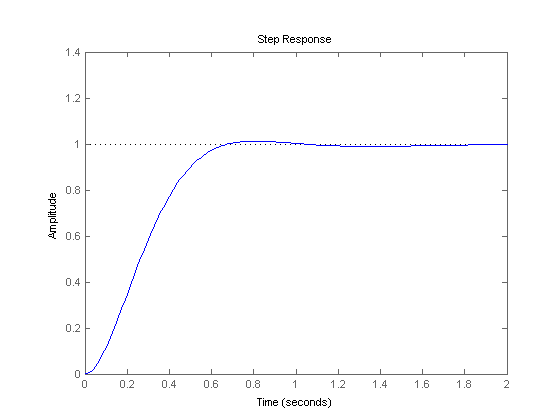
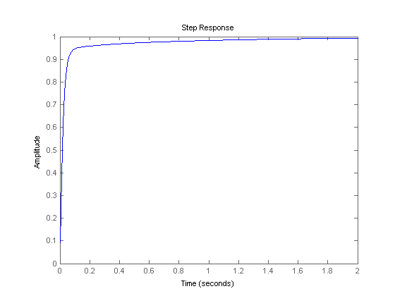
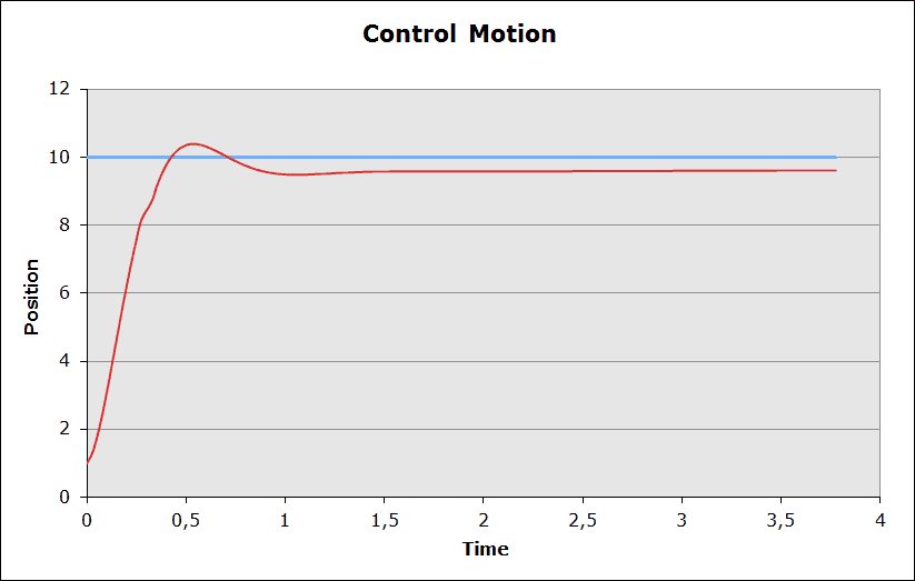
Another PID response plots:
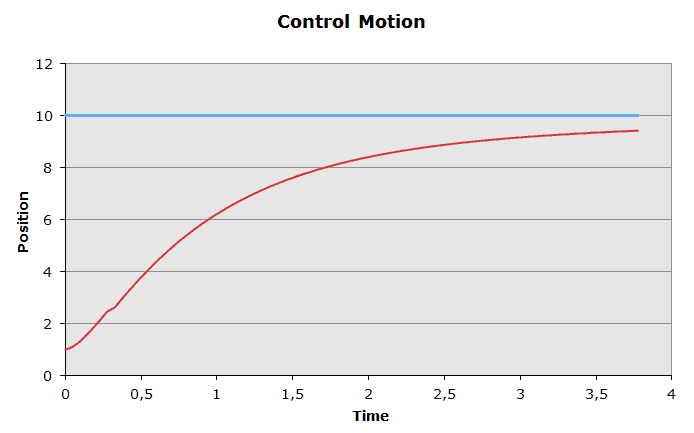
- Above: Very low Proportional and Integral factor. There is an offset between our goal and the output. Not very fast response (takes some time to reach the goal value)
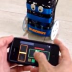
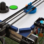
JJrobots projects using PID controllers:
We have been using PID controls extensively in our projects. A good example is the B-robot project. The PID are used here to solve the inverted pendulum problem.
Info / links / sources:
- http://www.csimn.com/CSI_pages/PIDforDummies.html (impressive documentation and graphs)
- http://en.wikipedia.org/wiki/PID_controller